Person Identification

There have been many implementations in recent years for identifying the human form within a given photo frame, however one particular method stands out called Histograms of Oriented Gradient (HOG) descriptors. Given a training set, the HOG algorithm is capable of eliminating information irrelevant to human detection. The human form can be shown in many different poses, perspective, ambient lighting and backgrounds, however one of the most important characteristics that is common to all are edges and corners. 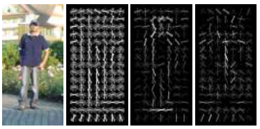The edge and gradient structure information is defined locally in small regions. The HOG technique consists of counting occurrences of gradient directions in localized cells (or pixel matrices). We then normalize these local histograms. It is suggested that the human form can be represented by using the distribution of local intensity gradients.

For my MATLAB implementation, check out my Github.

Implementation

The person identification system can be divided into two main functions which are:

• TrainHOG – will compute the necessary weights from training data.
• PredictHOG – will use the previously mentioned weights for predicting whether input images are human or not.

TrainHOG

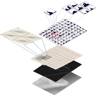
The function starts by reading the contents of the parameter file and obtaining a feature vector for each image within the training set. The HOG technique can be summed up in the following steps:

1. Image Normalization
   • Scaling images
   • Cropping. The given training set came with bounding box coordinates.
2. Colour Transformation
   • Coloured images consist of 3 channels (RGB), it is best to work with one channel.
   • In my tests, I converted everything to grayscale and achieved excellent results.
   • There are other colour spaces that are said to be better than grayscale such as CIELUV, CIELAB and CIEXYZ.
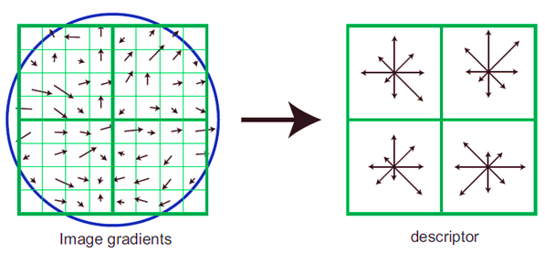
3. Gradient Computation
   • Generate the gradient for each pixel
4. Histogram Binning
   • Group pixels into cells.
   • Bin (count frequencies) pixels within the same cell based on direction.
5. Block Normalization
   • Group cells into blocks. N
   • Normalize each bin around the block.
   • Output each bin, for each cell as a feature.

After computing the feature vector for each image, we start training. What we are trying to achieve here is the ideal set of weights that can be used for training.

A classifier is required in order to classify examples. one excellent classifier would be logistic regression. Logistic regression follows what is known as a sigmoid function. The main advantage of using a sigmoid function is that the output would eventually be a probability between 0 and 1 (therefore, human or no human). Therefore this makes a much more ideal model to follow rather than linear regression, which is more suitable for defining relationships rather than classification. Classification in the sigmoid function can be done by setting a certain threshold, such as 0.5 and classifying values according to whether they are greater or smaller than this threshold.

So, from the training examples (which are divided into positive and negative examples) we know the input x (the feature vector) and we know the output (1/0, true/false, person/not a person). This leaves us no choice but to learn what is called the gradient descent.

The initial weight vector is set to 0. A learning function will then be set to iterate until it is stopped by a cost function. In each iteration, the gradient descent is calculated with the following formula: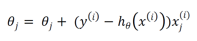Where j is the number of images, h is the sigmoid function and Θj the gradient descent, which needs to be iteratively trimmed. Using the gradient descent, we can then calculate the weights:

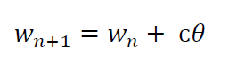
where ε is the learning rate and Θ the gradient descent.

The iterations (which by the way, have nothing to do with the number of images) can be terminated in two ways:

1. Setting a fixed number of iterations. (Personally, setting it to 200 iterations gave me the best result for 13,000 training images).
2. or using a cost function. (In the real world, this is ideal because it stops iterations when the function has learnt enough).

The following cost function was used:

PredictHOG

The PredictHOG function basically takes the outputted weights from the TrainHOG function, calculates the feature vector of the input image, and inputs these values within the sigmoid function. A certain probability value is returned. if it is greater than 0.5, then it images is labelled as true(is a person), otherwise false. Some statistical results are outputted to result.txt.

Conclusion

Results really depend on what parameters you put in. These parameters achieved 97% negative accuracy and 93% postive accuracy:

• Image resizing to 128×64 pixels
• Cell size of 9×9
• 16 bins
• Block size 5×5
• Overlap size (for blocks) 3×3
• Vector size of 10000
• learning rate 0.04

In some cases, using tanh x instead of the sigmoid function seemed to improve results slightly.